Camera Calibration - From 3D World to Image
Understanding the mathematics behind camera calibration and how 3D world points are transformed into 2D images
Introduction
Have you ever thought about how we capture the beautiful world? At least for me, it's quite mysteries. From a modern camera point of view, it transforms a point from a random world coordinate to camera frame coordinates, then to a 2D image with a certain pixel structure.
In this article, I'm going to talk about how these two transformations work mathematically.
Basic
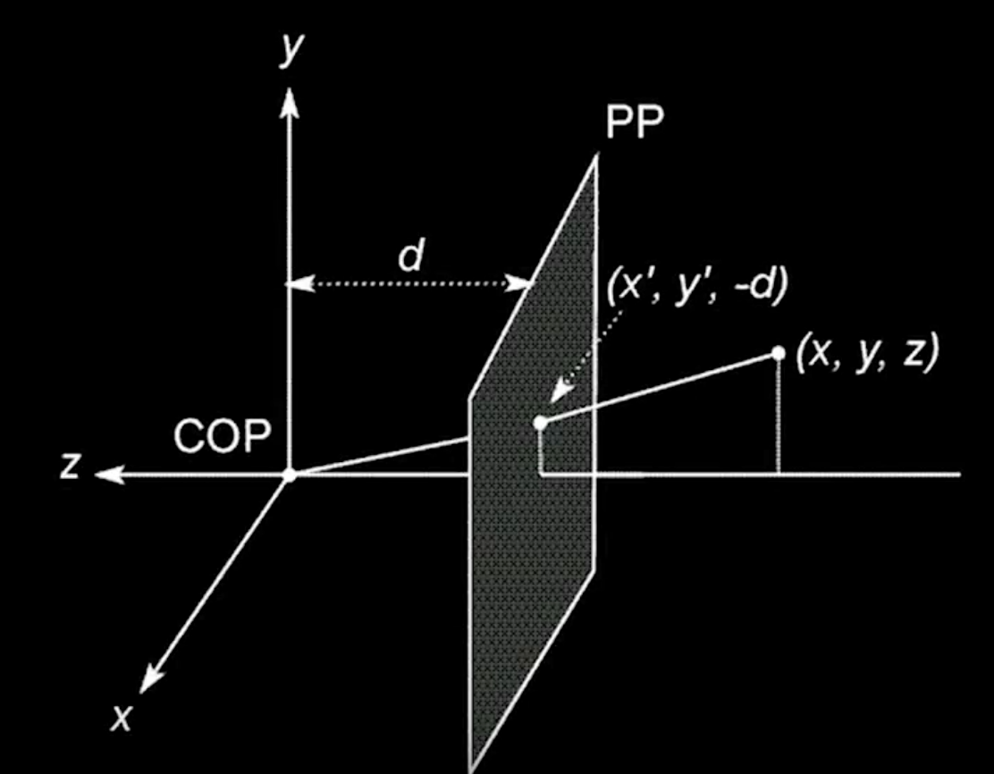
As the following image shows, is the basic projection model, which adopts the pinhole model as an approximation.
 Camera System
source
Camera System
source
Notations:
COPrefers to center of projection, also called optical center in the camera, which is the origin of our camera coordinate system.PPis the image plane in the camera frame.frefers to focal length, the distance betweenCOPto image plan (isdin the image above)
In this representation, we put the image plane in front of the camera coordinate system, to avoid mathematically flipping the image. As a result, we have x pointing right, y pointing up and z pointing inwards.
Now we can project a point in the world to image plane
, derived from similar triangles. The location on the image is just
by throwing out the z value.
Degree of Freedom
Mathematically, degrees of freedom is the number of dimensions of the domain of a random vector, or essentially the number of "free" components (how many components need to be known before the vector is fully determined).
We will use this term as DoF in the following transformation to measure each step.
Homogeneous Coordinates
Note that the operation by converting the location to is actually not a linear transformation because division by a non-constant
z is non-linear. For each point, z is an independent value thus the transformation will be done case by case. To fix this issue we introduce a new coordinate as follows:
The 1 we added is called a homogenous component of the vector, later we could also use other values.
Converting from the homogenous coordinates to non-homogenous one is quite easy, by dividing the value, the scale factor.
Now we could use matrix multiplication with homogenous coordinates to do the projection. (We mentioned f is the focal length.)
where you could think them as the pixel vectors on 2D image. We can also scale the projection matrix and get invariant result.
We will utilize homogenous coordinate system to do many powerful transformation in the following sections.
Camera Calibration
The geometric calibration will be divided into two parts - extrinsic and intrinsic.
The extrinsic part is about mapping from some arbitrary world coordinate system to the camera's 3D coordinate system, also called camera pose.
The intrinsic part is from 3D coordinates in the camera frame to the 2D image plane via projection.
Extrinsic Parameters
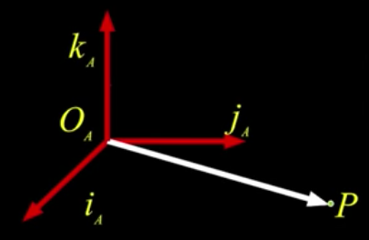
Before we talk about extrinsic parameters, we need to understand how we represent a point in a certain coordinate system.
 Coordinate System
source
Coordinate System
source
As the above picture shows, P is a point in coordinate A.
which is equivalent to
Translation
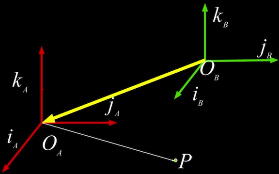
Now if we want to translate P from coordinate system A to B,
 Translation
source
Translation
source
we just use the location in coordinate system A plus the origin A represented in coordinate system B.
The rule also applies to another direction.
Fortunately, we learned from the last section that translation can be represented as a matrix multiplication using homogenous coordinates. Thus we have
which is equivalent to
where I is the 3x3 identity matrix.
There are 3 DoFs in translation.
Rotation
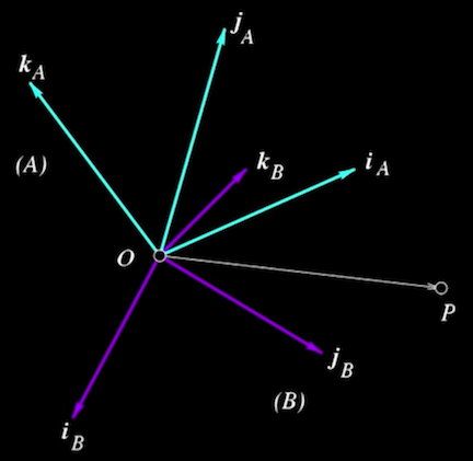
Besides translation, the point could also be rotated in another coordinate system like
 Combined Transformation
source
Combined Transformation
source
And we could represent it as
or
where describes frame A in the coordinate system of frame B.
Using homogenous coordinates, we can represent rotation as
There are 3 DoFs in rotation.
Rigid transformation
Combining the previous observations, we could unify them as
and
where is the transformation from A to B. In the other direction, we could have
The entire 4x4 is the extrinsic parameters matrix, finally!
Totally, we have 6 DoFs in extrinsic part.
Intrinsic Parameters
Remember in our homogenous coordinate section, we have a perspective projection, but the ideal version
It's ideal because in real world,
- pixels are in some arbitrary spatial units and
fis sometimes represented as pixels, thus we may use a scale factorto represent
f - pixel is not always square! We need another scale factor
.
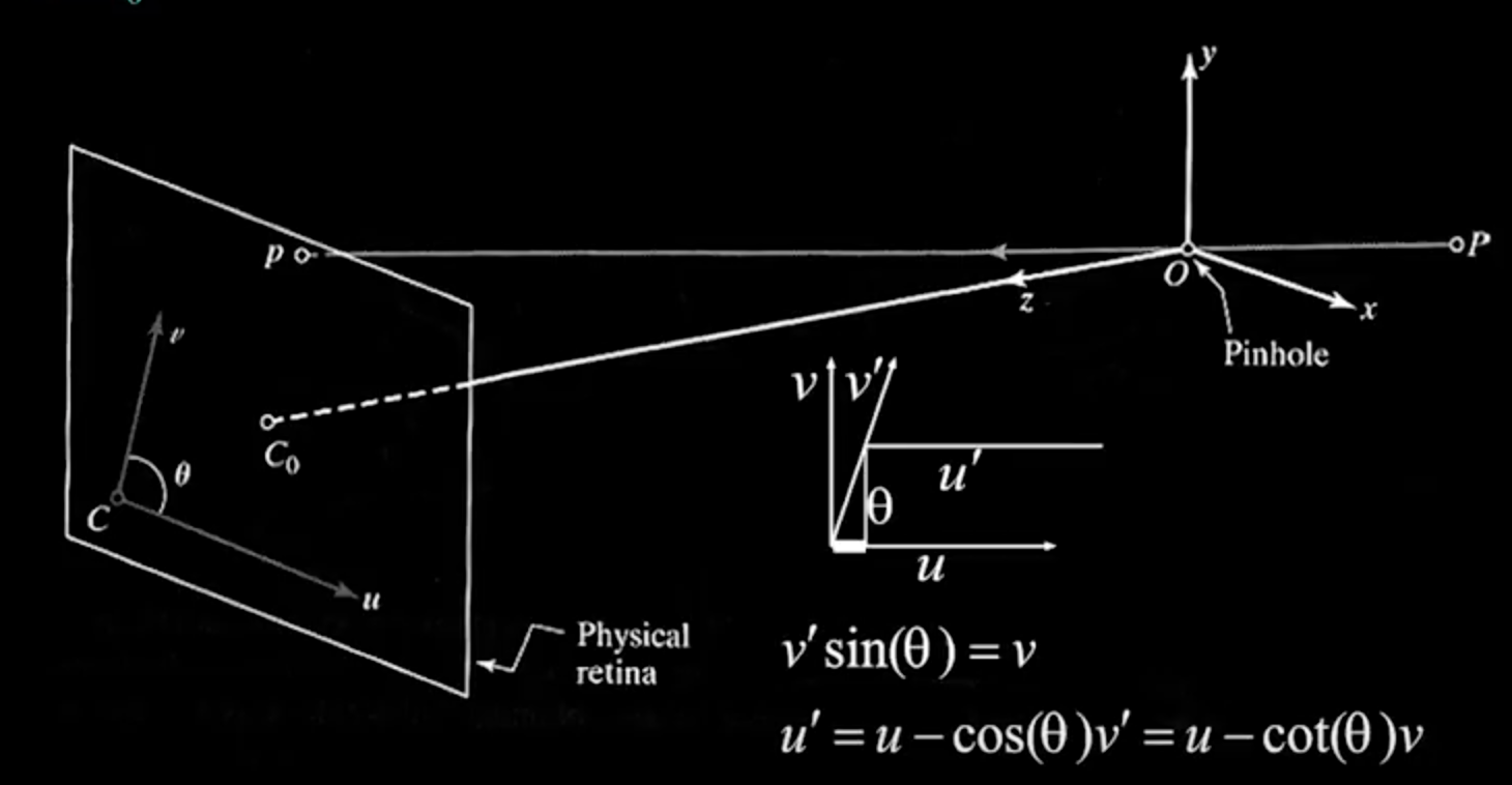
- pixel's axes may be skew
- optical center is not always the camera center, so we have two more offsets values to each dimension,
 Real World Camera
source
Real World Camera
source
And our pixel equation becomes
Now let's convert it to homogenous coordinates,
There are 6 DoFs in this model
We could use the simpler model as follows
where f is focal length, a is the ratio of u and v in f, and are the offsets. There are 5 DoFs.
The matrix taking a camera-based 3D coordinates to homogenous pixel coordinates is the intrinsic parameters.
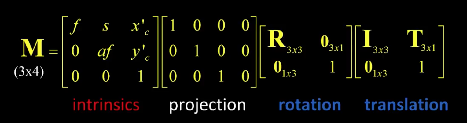
Combining them
We take all things together, translation, rotation, projection and intrinsics as our final camera parameters as follows. There are 11 DoFs.
 Complete Camera Model
source
Complete Camera Model
source
Reference
- Class materials from Introduction to Computer Vision by Georgia Tech & Udacity
- Degree of Freedom from Wiki